


Yun Yang and Ke Chen, Senior Member, IEEE
Abstract—
Temporal data clustering provides underpinning techniques for discovering the intrinsic structure and condensing information over temporal data. In this paper, we present a temporal data clustering framework via a weighted clustering ensemble of multiple partitions produced by initial clustering analysis on different temporal data representations. In our approach, we propose a novel weighted consensus function guided by clustering validation criteria to reconcile initial partitions to candidate consensus partitions from different perspectives, and then, introduce an agreement function to further reconcile those candidate consensus partitions to a final partition. As a result, the proposed weighted clustering ensemble algorithm provides an effective enabling technique for the joint use of different representations, which cuts the information loss in a single representation and exploits various information sources underlying temporal data. In addition, our approach tends to capture the intrinsic structure of a data set, e.g., the number of clusters. Our approach has been evaluated with benchmark time series, motion trajectory, and time-series data stream clustering tasks. Simulation results demonstrate that our approach yields favorite results for a variety of temporal data clustering tasks. As our
weighted cluster ensemble algorithm can combine any input partitions to generate a clustering ensemble, we also investigate its limitation by formal analysis and empirical studies.
Index Terms—Temporal data clustering, clustering ensemble, different representations, weighted consensus function, model
selection.
1 INTRODUCTION
TEMPORAL data are ubiquitous in the real world and there are many application areas ranging from multimedia information processing to temporal data mining. Unlike
static data, there is a high amount of dependency among temporal data and the proper treatment of data dependency or correlation becomes critical in temporal data processing.
Temporal clustering analysis provides an effective wayto discover the intrinsic structure and condense informationover temporal data by exploring dynamic regularities underlying temporal data in an unsupervised learning way. Its ultimate objective is to partition an unlabeled
temporal data set into clusters so that sequences grouped in the same cluster are coherent. In general, there are two core problems in clustering analysis, i.e., model selection andgrouping. The former seeks a solution that uncovers the number of intrinsic clusters underlying a temporal data set, while the latter demands a proper grouping rule that groups coherent sequences together to form a cluster matching an underlying distribution. Clustering analysis
is an extremely difficult unsupervised learning task. It is inherently an ill-posed problem and its solution often violates some common assumptions [1]. In particular, recent empirical studies [2] reveal that temporal data clustering poses a real challenge in temporal data mining due to the high dimensionality and complex temporal correlation. In the context of the data dependency treatment, we classify existing temporal data clustering algorithms as three
categories: temporal-proximity-based, model-based, and
representation-based clustering algorithms.
Temporal-proximity-based [2], [3], [4] and model-based
clustering algorithms [5], [6], [7] directly work on temporal
data. Therefore, temporal correlation is dealt with directly
during clustering analysis by means of temporal similarity
measures [2], [3], [4], e.g., dynamic time warping, or dynamic
models [5], [6], [7], e.g., hidden Markov model. In contrast, a
representation-based algorithm converts temporal data
clustering into static data clustering via a parsimonious
representation that tends to capture the data dependency.
Based on a temporal data representation of fixed yet
lower dimensionality, any existing clustering algorithm is
applicable to temporal data clustering, which is efficient in
computation. Various temporal data representations have
been proposed [8], [9], [10], [11], [12], [13], [14], [15] from
different perspectives. To our knowledge, there is no
universal representation that perfectly characterizes all
kinds of temporal data; one single representation tends to
encode only those features well presented in its own
representation space and inevitably incurs useful information
loss. Furthermore, it is difficult to select a representation
to present a given temporal data set properly without
prior knowledge and a careful analysis. These problems
often hinder a representation-based approach from achieving
the satisfactory performance.
As an emerging area in machine learning, clustering
ensemble algorithms have been recently studied from
IEEE TRANSACTIONS ON KNOWLEDGE AND DATA ENGINEERING, VOL. 23, NO. 2, FEBRUARY 2011 307
. The authors are with the School of Computer Science, The University of
Manchester, Kilburn Building, Oxford Road, Manchester M13 9PL, UK.
E-mail: yun.yang@postgrad.manchester.ac.uk, chen@cs.manchester.ac.uk.
Manuscript received 22 Jan. 2009; revised 3 July 2009; accepted 1 Nov. 2009;
published online 15 July 2010.
Recommended for acceptance by D. Papadias.
For information on obtaining reprints of this article, please send e-mail to:
tkde@computer.org, and reference IEEECS Log Number TKDE-2009-01-0033.
Digital Object Identifier no. 10.1109/TKDE.2010.112.
1041-4347/11/$26.00 2011 IEEE Published by the IEEE Computer Society
different perspective, e.g., clustering ensembles with graph
partitioning [16], [18], evidence aggregation [17], [19], [20],
[21], and optimization via semidefinite programming [22].
The basic idea behind clustering ensemble is combining
multiple partitions on the same data set to produce a
consensus partition expected to be superior to that of given
input partitions. Although there are few studies in
theoretical justification on the clustering ensemble methodology,
growing empirical evidences support such an idea,
and indicate that the clustering ensemble is capable of
detecting novel cluster structures [16], [17], [18], [19], [20],
[21], [22]. In addition, a formal analysis on clustering
ensemble reveals that under certain conditions, a proper
consensus solution uncovers the intrinsic structure underlying
a given data set [23]. Thus, clustering ensemble
provides a generic enabling technique to use different
representations jointly for temporal data clustering.
Motivated by recent clustering ensemble studies [16],
[17], [18] ,[19], [20], [21], [22], [23] and our success in the use
of different representations to deal with difficult pattern
classification tasks [24], [25], [26], [27], [28], we present an
approach to temporal data clustering with different
representations to overcome the fundamental weakness of
the representation-based temporal data clustering analysis.
Our approach consists of initial clustering analysis on
different representations to produce multiple partitions and
clustering ensemble construction to produce a final partition
by combining those partitions achieved in initial
clustering analysis. While initial clustering analysis can be
done by any existing clustering algorithms, we propose a
novel weighted clustering ensemble algorithm of a twostage
reconciliation process. In our proposed algorithm, a
weighting consensus function reconciles input partitions to
candidate consensus partitions according to various clustering
validation criteria. Then, an agreement function
further reconciles those candidate consensus partitions to
yield a final partition.
The contributions of this paper are summarized as
follows: First, we develop a practical temporal data
clustering model by different representations via clustering
ensemble learning to overcome the fundamental weakness
in the representation-based temporal data clustering analysis.
Next, we propose a novel weighted clustering ensemble
algorithm, which not only provides an enabling technique
to support our model but also can be used to combine any
input partitions. Formal analysis has also been done.
Finally, we demonstrate the effectiveness and the efficiency
of our model for a variety of temporal data clustering tasks
as well as its easy-to-use nature as all internal parameters
are fixed in our simulations.
In the rest of the paper, Section 2 describes the motivation
and our model, and Section 3 presents our weighted
clustering ensemble algorithm along with algorithm analysis.
Section 4 reports simulation results on a variety of temporal
data clustering tasks. Section 5 discusses issues relevant to
our approach, and the last section draws conclusions.
2 TEMPORAL DATA CLUSTERING WITH DIFFERENT
REPRESENTATIONS
In this section, we first describe our motivation to propose
our temporal data clustering model. Then, we present our
temporal data clustering model working on different
representations via clustering ensemble learning.
2.1 Motivation
It is known that different representations encode various
structural information facets of temporal data in their
representation space. For illustration, we perform the
principal component analysis (PCA) on four typical
representations (see Section 4.1 for details) of a synthetic
time-series data set. The data set is produced by the
stochastic function FðtÞ ¼ Asinð2 t þ BÞ þ "ðtÞ, where A,
B, and are free parameters and "ðtÞ is the added noise
drawn from the normal distribution N(0, 1). The use of four
different parameter sets (A, B, ) leads to time series of four
classes and 100 time series in each class.
As shown in Fig. 1, four representations of time series
present themselves with various distributions in their PCA
representation subspaces. For instance, both of classes
marked with triangle and star are easily separated from
other two overlapped classes in Fig. 1a, while so is the
classes marked with circle and dot in Fig. 1b. Similarly,
different yet useful structural information can also be
observed from plots in Figs. 1c and 1d. Intuitively, our
observation suggests that a single representation simply
captures partial structural information and the joint use of
different representations is more likely to capture the
intrinsic structure of a given temporal data set. When a
clustering algorithm is applied to different representations,
diverse partitions would be generated. To exploit all
information sources, we need to reconcile diverse partitions
to find out a consensus partition superior to any input
partitions.
From Fig. 1, we further observe that partitions yielded by
a clustering algorithm are unlikely to carry the equal
amount of useful information due to their distributions in
different representation spaces. However, most of existing
clustering ensemble methods treat all of partitions equally
308 IEEE TRANSACTIONS ON KNOWLEDGE AND DATA ENGINEERING, VOL. 23, NO. 2, FEBRUARY 2011
Fig. 1. Distributions of the time-series data set in various PCA
representation manifolds formed by the first two principal components
of their representations. (a) PLS. (b) PDWT. (c) PCF. (d) DFT.
during the reconciliation, which brings about an averaging
effect. Our previous empirical studies [29] found that such a
treatment could have the following adverse effects. As
partitions to be combined are radically different, the
clustering ensemble methods often yield a worse final
partition. Moreover, the averaging effect is particularly
harmful in a majority voting mechanism especially as many
highly correlated partitions appear highly inconsistent with
the intrinsic structure of a given data set. As a result, we
strongly believe that input partitions should be treated
differently so that their contributions would be taken into
account via a weighted consensus function.
Without the ground truth, the contribution of a partition
is actually unknown in general. Fortunately, existing
clustering validation criteria [30] measure the clustering
quality of a partition from different perspectives, e.g., the
validation of intra and interclass variation of clusters. To a
great extent, we can employ clustering validation criteria to
estimate contributions of partitions in terms of clustering
quality. However, a clustering validation criterion often
measures the clustering quality from a specific viewpoint
only by simply highlighting a certain aspect. In order to
estimate the contribution of a partition precisely in terms of
clustering quality, we need to use various clustering
validation criteria jointly. This idea is empirically justified
by a simple example below. In the following description, we
omit technical details of weighted clustering ensembles,
which will be presented in Section 3, for illustration only.
Fig. 2a shows a two-dimensional synthetic data set
subject to a mixture of Gaussian distribution where there
are five intrinsic clusters of heterogeneous structures, and
the ground truth partition is given for evaluation and
marked by diamond (cluster 1), light dot (cluster 2), dark
dot (cluster 3), square (cluster 4), and triangle (cluster 5).
The visual inspection on the structure of the data set shown
in Fig. 2a suggests that clusters 1 and 2 are relatively
separate, while cluster 3 spreads widely, and clusters 4 and
5 of different populations overlap each other.
Applying the K-mean algorithm on different initialization
conditions, including the center of clusters and the
number of clusters, to the data set yields 20 partitions. Using
different clustering validation criteria [30], we evaluate the
clustering quality of each single partition. Figs. 2b, 2c, and
2d depict single partitions of maximum value in terms of
different criteria. The DVI criterion always favors a partition
of balanced structure. Although the partition in Fig. 2b
meets this criterion well, it properly groups clusters 1-3 only
but fails to work on clusters 4 and 5. The MH criterion
generally favors partition with bigger number of clusters.
The partition in Fig. 2c meets this criterion but fails to group
clusters 1-3 properly. Similarly, the partition in Fig. 2d fails
to separate clusters 4 and 5 but is still judged as the best
partition in terms of the NMI criterion that favors the most
common structures detected in all partitions. By the use of a
single criterion to estimate the contribution of partitions in
the weight clustering ensemble (WCE), it inevitably leads to
incorrect consensus partitions, as illustrated in Figs. 2e, 2f,
and 2g, respectively. As three criteria reflect different yet
complementary facets of clustering quality, the joint use of
them to estimate the contribution of partitions becomes a
natural choice. As illustrated in Fig. 2h, the consensus
partition yielded by the multiple-criteria-based WCE is very
close to the ground truth in Fig. 2a. As a classic approach,
Cluster Ensemble [16] treats all partitions equally during
reconciling input partitions. When applied to this data set, it
yields a consensus partition shown in Fig. 2i that fails to
detect the intrinsic structure underlying the data set.
In summary, the above intuitive demonstration strongly
suggests the joint use of different representations for
temporal data clustering and the necessity of developing a
weighted clustering ensemble algorithm.
2.2 Model Description
Based on the motivation described in Section 2.1, we
proposed a temporal data clustering model with a weighted
clustering ensemble working on different representations.
As illustrated in Fig. 3, the model consists of three modules,
YANG AND CHEN: TEMPORAL DATA CLUSTERING VIA WEIGHTED CLUSTERING ENSEMBLE WITH DIFFERENT REPRESENTATIONS 309
Fig. 2. Results of clustering analysis and clustering ensembles. (a) The
data set of ground truth. (b) The partition of maximum DVI. (c) The
partition of maximum MH . (d) The partition of maximum NMI. (e) DVI
WCE. (f) MH WCE. (g) NMI WCE. (h) Multiple criteria WCE. (i) The
cluster ensemble [16].
Fig. 3. Temporal data clustering with different representations.
i.e., representation extraction, initial clustering analysis, and
weighted clustering ensemble.
Temporal data representations are generally classified
into two categories: piecewise and global representations. A
piecewise representation is generated by partitioning the
temporal data into segments at critical points based on a
criterion, and then, each segment will be modeled into a
concise representation. All segment representations in order
collectively form a piecewise representation, e.g., adaptive
piecewise constant approximation [8] and curvature-based
PCA segments [9]. In contrast, a global representation is
derived from modeling the temporal data via a set of basis
functions, and therefore, coefficients of basis functions
constitute a holistic representation, e.g., polynomial curve
fitting [10], [11], discrete Fourier transforms [13], [14], and
discrete wavelet transforms [12]. In general, temporal data
representations used in this module should be of the
complementary nature, and hence, we recommend the use
of both piecewise and global temporal data representations
together. In the representation extraction module, different
representations are extracted by transforming raw temporal
data to feature vectors of fixed dimensionality for initial
clustering analysis.
In the initial clustering analysis module, a clustering
algorithm is applied to different representations received
from the representation extraction module. As a result, a
partition for a given data set is generated based on each
representation. When a clustering algorithm of different
parameters is used, e.g., K-mean, more partitions based on a
representation would be produced by running the algorithm
on various initialization conditions. Thus, the clustering
analysis on different representations leads to multiple
partitions for a given data set. All partitions achieved will
be fed to the weighted clustering ensemble module for the
reconciliation to a final partition.
In the weighted clustering ensemble module, a weighted
consensus function works on three clustering validation
criteria to estimate the contribution of each partition received
from the initial clustering analysis module. The consensus
function with single-criterion-based weighting schemes
yields three candidate consensus partitions, respectively, as
presented in Section 3.1. Then, candidate consensus partitions
are fed to the agreement function consisting of a
pairwise majority voting mechanism, which will be presented
in Section 3.2, to form a final agreed partition where
the number of clusters is automatically determined.
3 WEIGHTED CLUSTERING ENSEMBLE
In this section, we first present the weight consensus
function based on clustering validation criteria, and then,
describe the agreement function. Finally, we analyze our
algorithm under the “mean” partition assumption made for
a formal clustering ensemble analysis [23].
3.1 Weighted Consensus Function
The basic idea of our weighted consensus function is the use
of the pairwise similarity between objects in a partition for
evident accumulation, where a pairwise similarity matrix is
derived from weighted partitions and weights are determined
by measuring the clustering quality with different
clustering validation criteria. Then, a dendrogram [3] is
constructed based on all similarity matrices to generate
candidate consensus partitions.
3.1.1 Partition Weighting Scheme
Assume that X ¼ fxngN
n¼1 is a data set of N objects and
there are M partitions P ¼ fPmgM
m¼1 on X, where the cluster
number in M partitions could be different, obtained from
the initial clustering analysis. Our partition weighting
scheme assigns a weight w
m to each Pm in terms of a
clustering validation criterion , and weights for all
partitions based on the criterion collectively form a
weight vector w ¼ fw
mgM
m¼1 for the partition collection P.
In the partition weighting scheme, we define a weight
w
m ¼
ðPmÞ
PM
m¼1 ðPmÞ
; ð1Þ
where w
m > 0 and
PM
m¼1 w
m ¼ 1. ðPmÞ is the clustering
validity index value in term of the criterion . Intuitively,
the weight of a partition would express its contribution to
the combination in terms of its clustering quality measured
by the clustering validation criterion .
As mentioned previously, a clustering validation criterion
measures only an aspect of clustering quality. In order
to estimate the contribution of a partition, we would
examine as many different aspects of clustering quality as
possible. After looking into all existing of clustering
validation criteria, we select three criteria of complementary
nature for generating weights from different perspectives as
elucidated below, i.e., Modified Huber’s index (MH )
[30], Dunn’s Validity Index (DVI) [30], and Normalized
Mutual Information (NMI) [16].
The MH index of a partition Pm [30] is defined by
MHTðPmÞ ¼
NðN 1Þ
2
XN 1
i¼1
XN
j¼iþ1
AijQij; ð2Þ
where Aij is the proximity matrix of objects and Q is an
N N cluster distance matrix derived from the partition
Pm, where each element Qij expresses the distance between
the centers of clusters to which xi and xj belong. Intuitively,
a high MH value for a partition indicates that the partition
has a compact and well-separated clustering structure.
However, this criterion strongly favors a partition containing
more clusters, i.e., increasing the number of clusters
results in a higher index value.
The DVI of a partition Pm [30] is defined by
DV IðPmÞ ¼ min
i;j
dðCm
i
; Cm
j Þ
maxk¼1;...;KmfdiamðCm
k Þg
; ð3Þ
where Cm
i , Cm
j , and Cm
k are clusters in Pm, dðCm
i ; Cm
j Þ is a
dissimilarity metric between clusters Cm
i and Cm
j , and
diamðCm
k Þ is the diameter of cluster Cm
k in Pm. Similar to the
MH index, the DVI also evaluates the clustering quality in
terms of compactness and separation properties. But it is
insensitive to the number of clusters in a partition. Nevertheless,
this index is less robust due to the use of a single
linkage distance and the diameter information of clusters,
e.g., it is quite sensitive to noise or outlier for any cluster of
a large diameter.
310 IEEE TRANSACTIONS ON KNOWLEDGE AND DATA ENGINEERING, VOL. 23, NO. 2, FEBRUARY 2011
The NMI [16] is proposed to measure the consistency
between two partitions, i.e., the amount of information
(common structured objects) shared between two partitions.
The NMI index for a partition Pm is determined by
summation of the NMI between the partition Pm and each
of other partitions Po. The NMI index is defined by
NMIðPm; PoÞ ¼
PKm
i¼1
PKo
j¼1 Nmo
ij log
NNmo
ij
Na
i Nb
j
PKm
i¼1 Nm
i log
Nm
i
N
þ
PKo
j¼1 No
j log
No
j
N
; ð4Þ
NMIðPmÞ ¼
XM
o¼1
NMIðPm; PoÞ: ð5Þ
Here, Pm and Po are two partitions that divide a data set of
N objects into Km and Ko clusters, respectively. Nmo
ij is the
number of shared objects between two different clusters
Cm
i 2 Pm and Co
j 2 Po, where there are Nm
i and No
j objects in
Cm
i and Co
j . Intuitively, a high NMI value implies a wellaccepted
partition that is more likely to reflect the intrinsic
structure of the given data set. This criterion biases toward
the highly correlated partitions and favors those clusters
containing a similar number of objects.
Inserting (2)-(5) into (1) by substituting for a specific
clustering validity index results in three weight vectors,
wMH , wDV I , and wNMI , respectively. They will be used to
weight the similarity matrix, respectively.
3.1.2 Weighted Similarity Matrix
For each partition Pm, a binary membership indicator
matrix Hm ¼ f0; 1gN Km is constructed where Km is the
number of clusters in the partition Pm. In the matrix Hm, a
row corresponds to one datum and a column refers to a
binary encoding vector for one specific cluster in the
partition Pm. Entities of column with one indicate that the
corresponding objects are grouped into the same cluster,
and zero otherwise. Now, we use the matrix Hm to derive
an N N binary similarity matrix Sm that encodes the
pairwise similarity between any two objects in a partition.
For each partition Pm, its similarity matrix Sm ¼ f0; 1gN N
is constructed by
Sm ¼ HmHT
m: ð6Þ
In (6), the element ðSmÞij is equal to the inner product
between rows i and j of the matrix Hm. Therefore, objects i
and j are grouped into the same cluster if the element
ðSmÞij ¼ 1, and in different clusters otherwise.
Finally, a weighted similarity matrix S concerning all the
partitions in P is constructed by a linear combination of
their similarity matrix Sm with their weight w
m as
S ¼
XM
m¼1
w
mSm: ð7Þ
In our algorithm, three weighted similarity matrices SMHT,
SDV I , and SNMI are constructed, respectively.
3.1.3 Candidate Consensus Partition Generation
A weighted similarity matrix S is used to reflect the
collective relationship among all data in terms of different
partitions and a clustering validation criterion . The
weighted similarity matrix actually tends to accumulate
evidence in terms of clustering quality, and hence, treats all
partitions differently. For robustness against noise, we do
not combine three weight similarity matrices directly, but
use them to yield three candidate consensus partitions.
Motivated by the idea in [19], we employ the dendrogram-
based similarity partitioning algorithm (DSPA) developed
in our previous work [29] to produce a candidate
consensus partition from a weighted similarity matrix S .
Our DSPA algorithm uses an average-link hierarchical
clustering algorithm that converts the weighted similarity
matrix into a dendrogram [3] where its horizontal axis
indexes all the data in a given data set, while its vertical axis
expresses the lifetime of all possible cluster formation. The
lifetime of a cluster in the dendrogram is defined as an
interval from the moment that the cluster is created to the
moment that it disappears by merging with other clusters.
Here, we emphasize that due to the use of a weighted
similarity matrix, the lifetime of clusters is weighted by the
clustering quality in terms of a specific clustering validation
criterion, and the dendrogram produced in this way is quite
different from that yielded by the similarity matrix without
being weighed [19].
As a consequence, the number of clusters in a candidate
consensus partition P can be determined automatically by
cutting the dendrogram derived from S to form clusters at
the longest lifetime. With the DSPA algorithm, we achieve
three candidate consensus partitions P , ¼ fMH ;DV I;
NMIg, in our algorithm.
3.2 Agreement Function
In our algorithm, the weighted consensus function yields
three candidate consensus partitions, respectively, according
to three different clustering validation criteria, as
described in Section 3.1. In general, these partitions are
not always consistent with each other (see Fig. 2, for
example), and hence, a further reconciliation is required for
a final partition as the output of our clustering ensemble.
In order to obtain a final partition, we develop an
agreement function by means of the evident accumulation
idea [19] again. A pairwise similarity S is constructed with
three candidate consensus partitions in the same way as
described in Section 3.1.2. That is, a binary membership
indicator matrix H is constructed from partition P , where
¼ fMH ;DV I;NMIg. Then, concatenating three H
matrices leads to an adjacency matrix consisting of all the
data in a given data set versus candidate consensus
partitions, H ¼ ½HMH jHDV I jHNMI . Thus, the pairwise
similarity matrix S is achieved by
S ¼
1
3
HHT : ð8Þ
Finally, a dendrogram is derived from S and the final
partition P is achieved with the DSPA algorithm [32].
3.3 Algorithm Analysis
Under the assumption that any partition of a given data set
is a noisy version of its ground truth partition subject to the
Normal distribution [23], the clustering ensemble problem
can be viewed as finding a “mean” partition of input
partitions in general. If we know the ground truth partition
YANG AND CHEN: TEMPORAL DATA CLUSTERING VIA WEIGHTED CLUSTERING ENSEMBLE WITH DIFFERENT REPRESENTATIONS 311
C and all possible partitions Pi of the given data set, the
ground truth partition would be the “mean” of all possible
partitions [23]:
C ¼ arg min
P
X
i
PrðPi ¼ CÞdðPi; PÞ; ð9Þ
where PrðPi ¼ CÞ is the probability that C is randomly
distorted to be Pi and dð ; Þ is a distance metric for any two
partitions. Under the Normal distribution assumption,
PrðPi ¼ CÞ is proportional to the similarity between Pi andC.
In a practical clustering ensemble problem, an initial
clustering analysis process returns only a partition subset
P ¼ fPmgM
m¼1. From (9), finding the “mean” P of M
partitions in P can be performed by minimizing the cost
function:
ðPÞ ¼
XM
m¼1
mdðPm; PÞ; ð10Þ
where m / PrðPm ¼ CÞ and
PM
m¼1 m ¼ 1. The optimal
solution to minimizing (10) is the intrinsic “mean” P :
P ¼ arg min
P
XM
m¼1
mdðPm; PÞ:
In this paper, we use the piecewise similarity matrix to
characterize a partition, and hence, define the distance as
dðPm; PÞ ¼ kSm Sk2, where S is the similarity matrix of a
consensus partition P. Thus, (10) can be rewritten as
ðPÞ ¼
XM
m¼1
mkSm Sk2: ð11Þ
Let S be the similarity matrix of the “mean” P . Finding P
to minimize ðPÞ in (11) is analytically solvable [31], i.e.,
S ¼
PM
m¼1 mSm. By connecting this optimal “mean” to the
cost function in (11), we have
ðPÞ ¼
XM
m¼1
mkSm Sk2
¼
XM
m¼1
mkðSm S Þ þ ðS SÞk2
¼
XM
m¼1
mkðSm S Þk2 þ
XM
m¼1
mkðS SÞk2:
ð12Þ
Note that the fact that
PM
m¼1 mkSm S k ¼ 0 is applied
in the last step of (12) due to
PM
m¼1 P m ¼ 1 and S ¼ M
m¼1 mSm. The actual cost of a consensus partition is
now decomposed into two terms in (12). The first term
corresponds to the quality of input partitions, i.e., how
close they are to the ground truth partition C solely
determined by an initial clustering analysis regardless of
clustering ensemble. In other words, the first term is
constant once the initial clustering analysis returns a
collection of partitions P. The second term is determined
by the performance of a clustering ensemble algorithm
that yields the consensus partition P, i.e., how close the
consensus partition is to the weighted “mean” partition.
Thus, (12) provides a generic measure to analyze a
clustering ensemble algorithm.
In our weighted clustering ensemble algorithm, a consensus
partition is an estimated “mean” characterized in a
generic form: S ¼
PM
m¼1 wmSm, where wm is w
m yielded by a
single clustering validation criterion , or wm produced by
the joint use of multiple criteria. By inserting the estimated
“mean” in the above form and the intrinsic “mean” into (12),
the second term of (12) becomes
XM
m¼1
m
XM
m¼1
ð m wmÞSm
2
: ð13Þ
From (13), it is observed that the quantities j m wmj
critically determine the performance of a weighted clustering
ensemble.
For clustering analysis, it has been assumed that an
underlying structure can be detected if it holds well-defined
cluster properties, e.g., compactness, separability, and
cluster stability [3], [4], [30]. We expect that such properties
can be measured by clustering validation criteria so thatwm is
as close to m as possible. In reality, the ground truth
partition is generally not available for a given data set.
Without the knowledge on m, it is impossible to formally
analyze how good clustering validation criteria are to
estimate intrinsic weights. Instead, we undertake empirical
studies to investigate its capacity and limitation of our
weighted clustering ensemble algorithm based on elaborately
designed synthetic data sets of the ground truth
information, which is presented in Appendix A that can be
found on the Computer Society Digital Library at http://doi.
ieeecomputersociety.org/10.1109/2010.112.
4 SIMULATION
For evaluation, we apply our approach to a collection of
time-series benchmarks for temporal data mining [32], the
CAVIAR visual tracking database [33], and the PDMC timeseries
data stream data set [34]. We first present the
temporal data representations used for time-series benchmarks
and the CAVIAR database in Section 4.1, and then,
report experimental setting and results for various temporal
data clustering tasks in Sections 4.2-4.4.
4.1 Temporal Data Representations
For the temporal data expressed as fxðtÞgT
t¼1 with a length of
T temporal data points, we use two piecewise representations,
piecewise local statistics (PLS) and piecewise discrete
wavelet transform (PDWT), developed in our previous work
[29] and two classical global representations, polynomial curve
fitting (PCF) and discrete Fourier transforms (DFTs), together.
4.1.1 PLS Representation
A window of the fixed size is used to block time series into a
set of segments. For each segment, the first- and secondorder
statistics are used as features of this segment. For
segment n, its local statistics n and n are estimated by
n ¼
1
jWj
XnjWj
t¼1þðn 1ÞjWj
xðtÞ; n ¼
ffiffiffiffiffiffiffiffiffiffiffiffiffiffiffiffiffiffiffiffiffiffiffiffiffiffiffiffiffiffiffiffiffiffiffiffiffiffiffiffiffiffififfiffiffiffiffiffiffiffiffiffiffiffiffi
1
jWj
XnjWj
t¼1þðn 1ÞjWj
½xðtÞ n 2
vuut
;
where jWj is the size of the window.
312 IEEE TRANSACTIONS ON KNOWLEDGE AND DATA ENGINEERING, VOL. 23, NO. 2, FEBRUARY 2011
4.1.2 PDWT Representation
Discrete wavelet transform (DTW) is applied to decompose
each segment via the successive use of low-pass and highpass
filtering at appropriate levels. At level j, high-pass
filters j
H encode the detailed fine information, while lowpass
filters j
L characterize coarse information. For the
nth segment, a multiscale analysis of J levels leads to a local
representation with all coefficients:
fxðtÞgnjWj
t¼ðn 1ÞjWj )
J
L;
j
H
J
j¼1
:
However, the dimension of this representation is the
window size jWj. For dimensionality reduction, we apply
Sammon mapping technique [35] by mapping wavelet
coefficients nonlinearly onto a prespecified low-dimensional
space to form our PDWT representation.
4.1.3 PCF Representation
In [9], time series is modeled by fitting it to a parametric
polynomial function
xðtÞ ¼ RtR þ R 1tR 1 þ þ 1t þ 0:
Here, rðr ¼ 0; 1; . . .;RÞ is the polynomial coefficient of the
Rth order. The fitting is carried out by minimizing a leastsquare
error criterion. All R þ 1 coefficients obtained via the
optimization constitute a PCF representation, a locationdependent
global representation.
4.1.4 DFT Representation
Discrete Fourier transforms have been applied to derive a
global representation of time series in frequency domain
[10]. The DFT of time series fxðtÞgT
t¼1 yields a set of Fourier
coefficients:
ad ¼
1
T
XT
t¼1
xðtÞ exp
j2 dt
T
; d¼ 0; 1; . . . ; T 1:
Then, we retain only few top d (d T) coefficients for
robustness against noise, i.e., real and imaginary parts,
corresponding to low frequencies collectively form a Fourier
descriptor, a location-independent global representation.
4.2 Time-Series Benchmarks
Time-series benchmarks of 16 synthetic or real-world timeseries
data sets [32] have been collected to evaluate timeseries
classification and clustering algorithms in the context
of temporal data mining. In this collection [32], the ground
truth, i.e., the class label of time series in a data set and the
number of classes K , is given and each data set is further
divided into the training and testing subsets for the
evaluation of a classification algorithm. The information
on all 16 data sets is tabulated in Table 1. In our simulations,
we use all 16 whole data sets containing both training and
test subsets to evaluate clustering algorithms.
In the first part of our simulations, we conduct three
types of experiments. First, we employ classic temporal
data clustering algorithms directly working on time series
to achieve their performance on the benchmark collection
used as a baseline yielded by temporal-proximity- and
model-based algorithm. We use the hierarchical clustering
(HC) algorithm [3] and the K-mean-based hidden Markov
Model (K-HMM) [5], while the performance of the K-mean
algorithm is provided by benchmark collectors. Next, our
experiment examines the performance on four representations
to see if the use of a single representation is enough to
achieve the satisfactory performance. For this purpose, we
employ two well-known algorithms, i.e., K-mean, an
essential algorithm, and DBSCAN [36], a sophisticated
density-based algorithm that can discover clusters of
arbitrary shape and is good at model selection. Last, we
apply our WCE algorithm to combine input partitions
yielded by K-mean, HC, and DBSCAN with different
representations during initial clustering analysis.
We adopt the following experimental settings for the first
two types of experiments. For clustering directly on
temporal data, we allow the K-HMM to use the correct
cluster number K and the results of K-mean were achieved
on the same condition. There is no parameter setting in HC.
For clustering on single representation, K is also used in
K-mean. Although DBSCAN does not need the prior
knowledge on a given data set, two parameters in the
algorithm need to be tuned for the good performance [36].
We follow suggestions in literature [36] to find the best
parameters for each data set by an exhausted search within
a proper parameter range. Given the fact that K-mean is
sensitive to initial conditions even though K is given, we
run the algorithm 20 times on each data set with different
initial conditions in two aforementioned experiments. As
results achieved are used for comparison to clustering
ensemble, we report only the best result for fairness.
For clustering ensemble, we do not use the prior knowledge
K in K-mean to produce partitions on different
representations to test its model selection capability. As a
result, we take the following procedure to produce a
partition with K-mean. With a random number generator
of uniform distribution, we draw a number within the range
K 2 K K þ 2ðK >0Þ. Then, the chosen number is
the K used in K-mean to produce a partition on an initial
condition. For each data set, we repeat the above procedure
to produce 10 partitions on a single representation so that
there are totally 40 partitions for combination as K-mean is
used for initial clustering analysis. As mentioned previously,
there is no parameter setting in the HC, and therefore, only
one partition is yielded for a given data set. Thus, we need to
combine only four partitions returned by the HC on different
YANG AND CHEN: TEMPORAL DATA CLUSTERING VIA WEIGHTED CLUSTERING ENSEMBLE WITH DIFFERENT REPRESENTATIONS 313
TABLE 1
Time-Series Benchmark Information [32]
representations for each data set. When DBSCAN is used in
initial clustering analysis on different representations, we
combine four best partitions of each data set achieved from
single-representation experiments mentioned above.
It is worth mentioning that for all representation-based
clustering in the aforementioned experiments, we always fix
those internal parameters on representations (see Section 4.1
for details) for all 16 data sets. Here, we emphasize that
there is no parameter tuning in our simulations.
As the same as used by the benchmark collectors [32], the
classification accuracy [37] is used for performance evaluation.
It is defined by
SimðC;PmÞ ¼
XK
i¼1
max
j f1;...;kg
2
jCi \ Pmjj
jCij þ jPmjj
!
K :
Here, C ¼ fCi; . . .CK g is a labeled data set that offers the
ground truth and Pm ¼ fPm1; . . . ; PmKg is a partition produced
by a clustering algorithm for the data set. For
reliability, we use two additional common evaluation criteria
for further assessment but report those results in Appendix B,
which can be found on the Computer Society Digital Library
at http://doi.ieeecomputersociety.org/10.1109/2010.112,
due to the limited space here.
Table 2 collectively lists all the results achieved in three
types of experiments. For clustering directly on temporal
data, it is observed from Table 2 that K-HMM, a modelbased
method, generally outperforms K-mean and HC,
temporal-proximity methods, as it has the best performance
on 10 out of 16 data sets. Given the fact that HC is capable
for finding a cluster number in a given data set, we also
report the model selection performance of HC with the
notation that is added behind the classification accuracy if
HC finds the correct cluster numbers. As a result, HC
manages to find the correct cluster number for four data
sets only, as shown in Table 2, which indicates the model
selection challenge in clustering temporal data of high
dimensions. It is worth mentioning that the K-HMM takes a
considerably longer time in comparison with other algorithms
including clustering ensembles.
With regard to clustering on single representations, it is
observed from Table 2 that there is no representation that
always leads to the best performance on all data sets no
matter which algorithm, K-mean or DBSCAN, is used and
the winning performance is achieved across four representations
for different data sets. The results demonstrate the
difficulty in choosing an effective representation for a given
temporal data set. From Table 2, we observe that DBSCAN
is generally better than K-mean algorithm on the appropriate
representation space and correctly detects the right
cluster number for 9 out of 16 data sets totally with
appropriate representations and the best parameter setup. It
implies that model selection on the single representation
space is rather difficult, given the fact that a sophisticated
algorithm does not perform well due to information loss in
the representation extraction.
From Table 2, it is evident that our proposed approach
achieves significantly better performance in terms of both
classification accuracy and model selection no matter which
algorithm is used in initial clustering analysis. It is observed
that our clustering ensemble combining input partitions
produced by a clustering algorithm on different representations
always outperforms the best partition yielded by the
same algorithm on single representations even though we
compare the averaging result of our clustering ensemble to
the best one on single representations when K-mean is used.
In terms of model selection, our clustering ensemble fails to
detect the right cluster numbers for two and one out of
16 data sets only, respectively, as K-mean and HC are used
for initiation clustering analysis, while the DBSCAN clustering
ensemble is successful for 10 of 16 data sets. For
comparison on all three types of experiments, we present
the best performance with the bold entries in Table 2. It is
observed that our approach achieves the best classification
accuracy for 15 out of 16 data sets given the fact that K-mean,
HC, and DBSCAN-based clustering ensembles achieve the
best performance for six, four, and five of out of 16 data sets,
respectively, and K-HMM working on raw time series yields
the best performance for the Adiac data set.
314 IEEE TRANSACTIONS ON KNOWLEDGE AND DATA ENGINEERING, VOL. 23, NO. 2, FEBRUARY 2011
TABLE 2
Classification Accuracy (in Percent) of Different Clustering Algorithms on Time-Series Benchmarks [32]
In our approach, an alternative clustering ensemble
algorithm can be used to replace our WCE algorithm. For
comparison, we employ three state-of-the-art algorithms
developed from different perspectives, i.e., Cluster Ensemble
(CE) [16], hybrid bipartite graph formulation (HBGF) algorithm
[18], and semidefinite-programming-based clustering ensemble
(SDP-CE) [22]. In our experiments, K-mean is used for initial
clustering analysis. Given the fact that all three algorithms
were developed without addressing model selection, we use
the correct cluster number of each data set K in K-mean.
Thus, 10 partitions for a single presentation are generated
with different initial conditions, and overall, there are
40 partitions to be combined for each data set. For our
WCE, we use exactly the same procedure for K-mean to
produce partitions described earlier where K is randomly
chosen from K 2 K K þ 2ðK >0Þ. For reliability,
we conduct 20 trials and report the average and the standard
deviation of classification accuracy rates.
Table 3 shows the performance of four clustering ensemble
algorithms where the notation is as same as used in Table 2. It
is observed from Table 3 that the SDP-CE, the HBGF, and
the CE algorithms win on five, two, and one data sets,
respectively, while ourWCEalgorithm has the best results for
the remaining eight data sets. Moreover, a closer observation
indicates that our WCE algorithm also achieves the second
best results for four out of eight data sets where other
algorithms win. In terms of computational complexity, the
SDP-CE suffers from the highest computational burden,
while our WCE has higher computational cost than the CE
and the HBGF. Considering its capability of model selection
and a trade-off between performance and computational
efficiency, we believe that our WCE algorithm is especially
suitable for temporal data clustering with different representations.
Further assessment with other common evaluation
criteria is also done, and the entirely consistent results
reported in Appendix B, which can be found on the Computer
Society Digital Library at http://doi.ieeecomputersociety.
org/10.1109/2010.112, allow us to draw the same conclusion.
In summary, our approach yields favorite results on the
benchmark time-series collection in comparison to classical
temporal data clustering and the state-of-the-art clustering
ensemble algorithms. Hence, we conclude that our proposed
approach provides a promising yet easy-to-use technique for
temporal data mining tasks.
4.3 Motion Trajectory
In order to explore a potential application, we apply our
approach to the CAVIAR database for trajectory clustering
analysis. The CAVIA database [33] was originally designed
for video content analysis where there are the manually
annotated video sequences of pedestrians, resulting in
222 motion trajectories, as illustrated in Fig. 4.
Aspatiotemporal motion trajectory is a 2Dspatiotemporal
data of the notationfðxðtÞ; yðtÞÞgT
t¼1, where ðxðtÞ; yðtÞÞ is the
coordinates of an object tracked at frame t, and therefore, can
also be treated as two separate time series fxðtÞgT
t¼1 and
fyðtÞgT
t¼1 by considering its x- and y-projection, respectively.
As a result, the representation of a motion trajectory is simply
a collective representation of two time series corresponding
to its x- and y-projection. Motion trajectories tend to have the
various lengths, and therefore, a normalization technique
needs to be used to facilitate the representation extraction.
Thus, the motion trajectory is resampled with a prespecified
number of sample points, i.e., the length is 1,500 in our
simulations, by a polynomial interpolation algorithm. After
resampling, all trajectories are normalized to a Gaussian
distribution of zero mean and unit variance in x- and ydirections.
Then, four different representations described in
Section 4.1 are extracted from the normalized trajectories.
Given that there is no prior knowledge on the “right”
number of clusters for this database, we run the K-mean
algorithm 20 times by randomly choosing a K value from an
interval between five and 25 and initializing the center of a
cluster randomly to generate 20 partitions on each of four
representations. Totally, 80 partitions are fed to our WCE to
yield a final partition, as shown in Fig. 5. Without the
ground truth, human visual inspection has to be applied for
evaluating the results, as suggested in [38]. By the common
human visual experience, behaviors of pedestrians across
the shopping mall are roughly divided into five categories:
“move up,” “move down,” “stop,” “move left,” and “move
right” from the camera viewpoint [35]. Ideally, trajectories
of the similar behaviors are grouped together along a
motion direction, and then, results of clustering analysis are
used to infer different activities at a semantic level, e.g.,
“enter the store,” “exit from the store,” “pass in front,” and
“stop to watch.”
As observed from Fig. 5, coherent motion trajectories have
been properly grouped together, while dissimilar ones are
distributed into different clusters. For example, the trajectories
corresponding to the activity of “stop to watch” are
accurately grouped in the cluster shown in Fig. 5e. Those
trajectories corresponding to moving from left-to-right and
right-to-left are properly grouped into two separate clusters,
YANG AND CHEN: TEMPORAL DATA CLUSTERING VIA WEIGHTED CLUSTERING ENSEMBLE WITH DIFFERENT REPRESENTATIONS 315
TABLE 3
Classification Accuracy (in Percent) of Clustering Ensembles
Fig. 4. All motion trajectories in the CAVIA database.
as shown in Figs. 5c and 5f. The trajectories corresponding to
“move up” and “move down” are grouped into two clusters
as shown in Figs. 5j and 5k very well. Figs. 5a, 5d, 5g, 5h, 5i,
5n, and 5o indicate that trajectories corresponding to most
activities of “enter the store” and “exit from the store” are
properly grouped together via multiple clusters in light of
various starting positions, locations, moving directions, and
so on. Finally, Figs. 5l and 5m illustrate two clusters roughly
corresponding to the activity “pass in front.”
The CAVIAR database was also used in [38] where the
self-organizing map with the single DFT representation was
used for clustering analysis. In their simulation, the number
of clusters was determined manually and all trajectories
were simply grouped into nine clusters. Although most of
clusters achieved in their simulation are consistent with
ours, their method failed to separate a number of
trajectories corresponding to different activities by simply
putting them together into a cluster called “abnormal
behaviors” instead. In contrast, ours properly groups them
into several clusters, as shown in Figs. 5a, 5b, 5e, and 5i. If
the clustering analysis results are employed for modeling
events or activities, their merged cluster inevitably fails to
provide any useful information for a higher level analysis.
Moreover, the cluster shown in Fig. 5j, corresponding to
“move up,” was missing in their partition without any
explanation [38]. Here, we emphasize that unlike their
manual approach to model selection, our approach automatically
yields 15 meaningful clusters as validated by
human visual inspection.
To demonstrate the benefit from the joint use of different
representations, Fig. 6 illustrates several meaningless clusters
of trajectories, judged by visual inspection, yielded by
the same clustering ensemble but on single representations,
respectively. Figs. 6a and 6b show that using only the PCF
representation, some trajectories of line structures along xand
y-axis are improperly grouped together. For these
trajectories “perpendicular” to each other, their x and
y components have only a considerable coefficient value
on their linear basis but a tiny coefficient value on any higher
order basis. Consequently, this leads to a short distance
between such trajectories in the PCF representation space,
which is responsible for improper grouping. Figs. 6c and 6d
illustrate a limitation of the DFT representation, i.e.,
trajectories with the same orientation but with different
starting points are improperly grouped together since the
DFT representation is in the frequency domain, and therefore,
independent of spatial locations. Although the PLS and
PDWT representations highlight local features, global
characteristics of trajectories could be neglected. The cluster
based on the PLS representation shown in Fig. 6e improperly
groups trajectories belonging to two clusters in Figs. 5k
and 5n. Likewise, Fig. 6f shows an improper grouping based
on the PDWT representation that merges three clusters in
Figs. 5a, 5d, and 5i. All above results suggest that the joint
use of different representations is capable of overcoming
limitations of individual representations.
For further evaluation, we conduct two additional
simulations. The first one intends to test the generalization
performance on noisy data produced by adding different
amount of Gaussian noise Nð0; Þ to the range of coordinates
of moving trajectories. The second one tends to
simulate a scenario that a moving object tracked is occluded
by other objects or the background, which leads to missing
data in a trajectory. For the robustness, 50 independent
trials have been done in our simulations.
Table 4 presents results of classifying noisy trajectories
with the final partition, as shown in Fig. 5, where a decision
is made by finding a cluster whose center is closest to the
tested trajectory in terms of the euclidean distance to see if its
clean version belongs to this cluster. Apparently, the
classification accuracy highly depends on the quality of
clustering analysis. It is evident from Table 4 that the
performance is satisfactory in contrast to those of the
clustering ensemble on a single representation especially
316 IEEE TRANSACTIONS ON KNOWLEDGE AND DATA ENGINEERING, VOL. 23, NO. 2, FEBRUARY 2011
Fig. 6. Typical clustering results with a single representation only.
Fig. 5. The final partition on the CAVIAR database by our approach; (a),
(b), (c), (d), (e), (f), (g), (h), (i), (j), (k), (l), (m ), (n), and (o) plots
correspond to 15 clusters of moving trajectories.
as a substantial amount of noise is added, which again
demonstrates the synergy between different representations.
To simulate trajectories of missing data, we remove five
segments of trajectory of the identical length at random
locations, and missing segments of various lengths are used
for testing. As a result, the task is to classify a trajectory of
missing data with its observed data only and the same
decision-making rule mentioned above is used. We conduct
this simulation on all trajectories of missing data and their
noisy version by adding the Gaussian noise Nð0; 0:1Þ. Fig. 7
shows the performance evolution in the presence of missing
data measured by a percentage of the trajectory length. It is
evident that our approach performs well in simulated
occlusion situations.
4.4 Time-Series Data Stream
Unlike temporal data collected prior to processing, a data
stream consisting of variables continuously comes from a
data flow of a given source, e.g., sensor networks [34], at a
high speed to generate examples over time. The temporal
data stream clustering is a task finding groups of variables
that behave similarly over time. The nature of temporal data
streams poses a new challenge for traditional temporal
clustering algorithms. Ideally, an algorithm for temporal
data stream clustering needs to deal with each example in
constant time and memory [39].
Time-series data stream clustering has been recently
studied, e.g., an Online Divisive-Agglomerative Clustering
(ODAC) algorithm [39]. As a result, most of such algorithms
developed to work on a stream fragment to fulfill clustering
in constant time and memory. In order to exploit the potential
yet hidden information and to demonstrate the capability of
our approach in temporal data stream clustering, we propose
to use dynamic properties of a temporal data stream along
with itself together. It is known that dynamic properties of
time series, xðtÞ, can be well described by its derivatives of
different orders, xðnÞðtÞ; n ¼ 1; 2; . . . . As a result, we would
treat derivatives of a stream fragment and itself as different
representations, and then, use them for initial clustering
analysis in our approach. Given the fact that the estimate of
the nth derivative requires only n þ 1 successive points, a
slightly larger constant memory is used in our approach, i.e.,
for the nth order derivative of time series, the size of our
memory is n points larger than the size of the memory used
by the ODAC algorithm [39].
In our simulations, we use the PDMC Data Set collected
from streaming sensor data of approximately 10,000 hours of
time-series data streams containing several variables including
userID, sessionID, sessionTime, two characteristics,
annotation, gender, and nine sensors [34]. Following the
exactly same experimental setting in [39], we use theirODAC
algorithm for initial clustering analysis on three representations,
i.e., time series xðtÞ, and its first- and second-order
derivatives xð1ÞðtÞ and xð2ÞðtÞ. The same criteria, MH and
DVI, used in [39] are adopted for performance evaluation.
Doing so allows us to compare our proposed approach with
this state-of-the-art technique straightforward and to demonstrate
the performance gain by our approach via the
exploitation of hidden yet potential information.
As a result, Table 5 lists simulation results of our
proposed approach against those reported in [39] on two
collections, userID ¼ 6 of 80,182 observations and userID ¼
25 of 141,251 observations, for the task finding the right
number of clusters on eight sensors from 2 to 9. The best
results on two collections were reported in [39] where their
ODAC algorithm working on the time-series data streams
only found three sensor clusters for each user and their
clustering quality was evaluated by the MH and the DVI.
From Table 5, it is observed that our approach achieves
much higher MH and DVI values, but finds considerably
different cluster structures, i.e., five clusters found for
userID ¼ 6 and four clusters found for userID ¼ 25.
Although our approach considerably outperforms the
ODAC algorithm in terms of clustering quality criteria, we
would not conclude that our approach is much better than
the ODAC algorithm, given the fact that those criteria
evaluate the clustering quality from a specific perspective
only and there is no ground truth available. We believe that
a whole stream of all observations should contain the precise
information on its intrinsic structure. In order to verify our
results, we apply a batch hierarchical clustering (BHC)
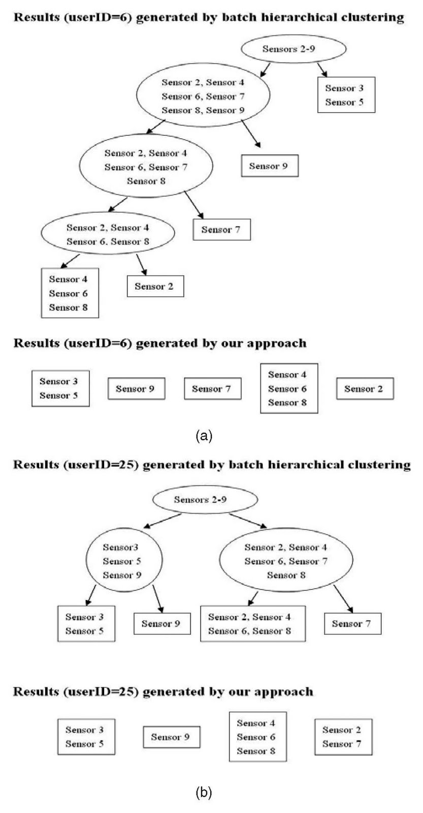
algorithm [3] to two pooled whole streams. Fig. 8 depicts
results of the batch clustering algorithm in contrast to ours.
It is evident that ours is completely consistent with that of
the BHC on userID ¼ 6, and ours on userID ¼ 25 is identical
to that of the BHC except that ours groups sensors 2 and 7 in
a cluster, but the BHC separates them and merges sensor 2 to
a larger cluster. Comparing with the structures uncovered
YANG AND CHEN: TEMPORAL DATA CLUSTERING VIA WEIGHTED CLUSTERING ENSEMBLE WITH DIFFERENT REPRESENTATIONS 317
Fig. 7. Classification accuracy of our approach on the CAVIAR database
and its noisy version in simulated occlusion situations.
TABLE 5
Results of the ODAC Algorithm versus Our Approach
TABLE 4
Performance on the CAVIAR Corrupted with Noise
by the ODAC [39], one can clearly see that theirs are quite
distinct from those yielded by the BHC algorithm. Although
our partition on userID ¼ 25 is not consistent with that of the
BHC, the overall results on two streams are considerably
better than those of the ODAC [39].
In summary, the simulation described above demonstrates
how our approach is applied to an emerging
application field in temporal data clustering. By exploiting
the additional information, our approach leads to a
substantial improvement. Using the clustering ensemble
with different representations, however, our approach has a
higher computational burden and requires a slightly larger
memory for initial clustering analysis. Nevertheless, it is
apparent from Fig. 3 that the initial clustering analysis on
different representations is completely independent and so
is the generation of candidate consensus partitions. Thus,
we firmly believe that the advanced computing technology
nowadays, e.g., parallel computation, can be adopted to
overcome the weakness for a real application.
5 DISCUSSION
The use of different temporal data representations in our
approach plays an important role in cutting information
loss during representation extraction, a fundamental weakness
of the representation-based temporal data clustering.
Conceptually, temporal data representations acquired from
different domains, e.g., temporal versus frequency, and on
different scales, e.g., local versus global as well as fine
versus coarse, tend to be complementary. In our simulations
reported in this paper, we simply use four temporal
data representations of a complementary nature to demonstrate
our idea in cutting information loss. Although our
work is concerning the representation-based clustering, we
have addressed little on the representation-related issues
per se including the development of novel temporal data
representations and the selection of representations to
establish a synergy to produce appropriate partitions for
clustering ensemble. We anticipate that our approach
would be improved once those representation-related
problems are tackled effectively.
The cost function derived in (12) suggests that the
performance of a clustering ensemble depends on both
quality of input partitions and a clustering ensemble
scheme. First, initial clustering analysis is a key factor
responsible for the performance. According to the first term
of (12) in Section 3.3, the good performance demands the
property that the variance of input partitions is small and
the optimal “mean” is close to the intrinsic “mean,” i.e., the
ground truth partition. Hence, appropriate clustering
algorithms need to be chosen to match the nature of a
given problem to produce input partitions of such a
property, apart from the use of different representations.
When domain knowledge is available, it can be integrated
via appropriate clustering algorithms during initial clustering
analysis. Moreover, the structural information underlying
a given data set may be exploited, e.g., via manifold
clustering [40], to produce input partitions reflecting its
intrinsic structure. As long as an initial clustering analysis
returns input partitions encoding domain knowledge and
characterizing the intrinsic structural information, the
“abstract” similarity (i.e., whether or not two entities are
in the same cluster) used in our weighted clustering
ensemble will inherit them during combination of input
partitions. In addition, the weighting scheme in our
algorithm also allows any other useful criteria and domain
knowledge to be integrated. All discussed above pave a
new way to improve our approach.
As demonstrated, a clustering ensemble algorithm
provides an effective enabling technique to use different
representations in a flexible yet effective way. Our previous
work [24], [25], [26], [27], [28] shows that a single learning
model working on a composite representation formed by
lumping different representations together is often inferior
to an ensemble of multiple learning models on different
representations for supervised and semisupervised learning.
Moreover, our earlier empirical studies [29] and those
318 IEEE TRANSACTIONS ON KNOWLEDGE AND DATA ENGINEERING, VOL. 23, NO. 2, FEBRUARY 2011
Fig. 8. Results of the batch hierarchical clustering algorithm versus ours
on two data stream collections. (a) userID ¼ 6. (b) userID ¼ 25.
not reported here also confirm our previous finding for
temporal data clustering. Therefore, our approach is more
effective and efficient than a single learning model on the
composite representation of a much higher dimension.
As a generic technique, our weighted clustering ensemble
algorithm is applicable to combination of any input
partitions in its own right regardless of temporal data
clustering. Therefore, we would link our algorithm to the
most relevant work and highlight the essential difference
between them.
The Cluster Ensemble algorithm [16] presents three
heuristic consensus functions to combine multiple partitions.
In their algorithm [16], three consensus functions are
applied to produce three candidate consensus partitions,
respectively, and then, the NMI criterion is employed to
find out a final partition by selecting the one of the
maximum NMI value from candidate consensus partitions.
Although there is a two-stage reconciliation process in both
their algorithm [16] and ours, the following characteristics
distinguish ours from theirs. First, ours uses only a uniform
weighted consensus function that allows various clustering
validation criteria for weight generation. Various clustering
validation criteria are used to produce multiple candidate
consensus partitions (in this paper, we use only three
criteria). Then, we use an agreement function to generate a
final partition by combining all candidate consensus
partitions other than selection.
Our consensus and the agreement functions are developed
under the evidence accumulation framework [19].
Unlike the original algorithm [19] where all input partitions
are treated equally, we use the evidence accumulated in a
selective way. When (13) is applied to the original algorithm
[19] for analysis, it can be viewed as a special case of our
algorithm as wm ¼ 1=M. Thus, its cost defined in (12) is
simply a constant independent of combination. In other
words, the algorithm in [19] does not exploit the useful
information on relationship between input partitions and
works well only if all input partition has a similar distance
to the ground truth partition in the partition space. Thus,
we believe that this analysis justifies the fundamental
weakness of a clustering ensemble algorithm, treating all
input partitions equally during combination.
Alternative weighted clustering ensemble algorithms
[41], [42], [43] have also been developed. In general, they
can be divided into two categories in terms of the weighting
scheme: cluster versus partition weighting. A cluster
weighting scheme [41], [42] associates clusters in a partition
with an weighting vector and embeds it in the subspace
spanned by an adaptive combination of feature dimensions,
while a partition weighting scheme [43] assigns a weight
vector to partitions to be combined. Our algorithm clearly
belongs to the latter category but adopts a different
principle from that used in [43] to generate weights.
The algorithm in [43] comes up with an objective
function encoding the overall weighted distance between
all input partitions to be combined and the consensus
partition to be found. Thus, an optimization problem has to
be solved to find the optimal consensus partition. According
to our analysis in Section 3.3, however, the optimal
“mean” in terms of their objective function may be insistent
with the optimal “mean” by minimizing the cost function
defined in (11), and here, the quality of their consensus
partition is not guaranteed. Although their algorithm is
developed under the nonnegative matrix factorization
framework [43], the iterative procedure for the optimal
solution incurs a high computational complexity of Oðn3Þ.
In contrast, our algorithm calculates weights directly with
clustering validation criteria, which allows for the use of
multiple criteria to measure the contribution of partitions
and leads to a much faster computation. Note that the
efficiency issue is critical for some real applications, e.g.,
temporal data stream clustering. In our ongoing work, we
are developing a weighting scheme of the synergy between
cluster and partition weighting.
6 CONCLUSION
In this paper, we have presented a temporal data clustering
approach via a weighted clustering ensemble on different
representations and further propose a useful measure to
understand clustering ensemble algorithms based on a
formal clustering ensemble analysis [23]. Simulations show
that our approach yields favorite results for a variety of
temporal data clustering tasks in terms of clustering quality
and model selection. As a generic framework, our weighted
clustering ensemble approach allows other validation
criteria [30] to be incorporated directly to generate a new
weighting scheme as long as they better reflect the intrinsic
structure underlying a data set. In addition, our approach
does not suffer from a tedious parameter tuning process
and a high computational complexity. Thus, our approach
provides a promising yet easy-to-use technique for realworld
applications.
ACKNOWLEDGMENTS
The authors are grateful to Vikas Singh who provides their
SDP-CE [22] Matlab code used in our simulations and
anonymous reviewers for their comments that significantly
improve the presentation of this paper. The Matlab code of
the CE [16] and the HBGF [18] used in our simulations was
downloaded from authors’ website.
REFERENCES
[1] J. Kleinberg, “An Impossible Theorem for Clustering,” Advances in
Neural Information Processing Systems, vol. 15, 2002.
[2] E. Keogh and S. Kasetty, “On the Need for Time Series Data
Mining Benchmarks: A Survey and Empirical Study,” Knowledge
and Data Discovery, vol. 6, pp. 102-111, 2002.
[3] A. Jain, M. Murthy, and P. Flynn, “Data Clustering: A Review,”
ACM Computing Surveys, vol. 31, pp. 264-323, 1999.
[4] R. Xu and D. Wunsch, II, “Survey of Clustering Algorithms,” IEEE
Trans. Neural Networks, vol. 16, no. 3, pp. 645-678, May 2005.
[5] P. Smyth, “Probabilistic Model-Based Clustering of Multivariate
and Sequential Data,” Proc. Int’l Workshop Artificial Intelligence and
Statistics, pp. 299-304, 1999.
[6] K. Murphy, “Dynamic Bayesian Networks: Representation,
Inference and Learning,” PhD thesis, Dept. of Computer Science,
Univ. of California, Berkeley, 2002.
[7] Y. Xiong and D. Yeung, “Mixtures of ARMA Models for Model-
Based Time Series Clustering,” Proc. IEEE Int’l Conf. Data Mining,
pp. 717-720, 2002.
[8] N. Dimitova and F. Golshani, “Motion Recovery for Video
Content Classification,” ACM Trans. Information Systems, vol. 13,
pp. 408-439, 1995.
[9] W. Chen and S. Chang, “Motion Trajectory Matching of Video
Objects,” Proc. SPIE/IS&T Conf. Storage and Retrieval for Media
Database, 2000.
YANG AND CHEN: TEMPORAL DATA CLUSTERING VIA WEIGHTED CLUSTERING ENSEMBLE WITH DIFFERENT REPRESENTATIONS 319
[10] C. Faloutsos, M. Ranganathan, and Y. Manolopoulos, “Fast
Subsequence Matching in Time-Series Databases,” Proc. ACM
SIGMOD, pp. 419-429, 1994.
[11] E. Sahouria and A. Zakhor, “Motion Indexing of Video,” Proc.
IEEE Int’l Conf. Image Processing, vol. 2, pp. 526-529, 1997.
[12] C. Cheong, W. Lee, and N. Yahaya, “Wavelet-Based Temporal
Clustering Analysis on Stock Time Series,” Proc. Int’l Conf.
Quantitative Sciences and Its Applications, 2005.
[13] E. Keogh, K. Chakrabarti, M. Pazzani, and S. Mehrota, “Locally
Adaptive Dimensionality Reduction for Indexing Large Scale
Time Series Databases,” Proc. ACM SIGMOD, pp. 151-162, 2001.
[14] F. Bashir, “MotionSearch: Object Motion Trajectory-Based Video
Database System—Index, Retrieval, Classification and Recognition,”
PhD thesis, Dept. of Electrical Eng., Univ. of Illinois,
Chicago, 2005.
[15] E. Keogh and M. Pazzani, “A Simple Dimensionality Reduction
Technique for Fast Similarity Search in Large Time Series
Databases,” Proc. Pacific-Asia Conf. Knowledge Discovery and Data
Mining, pp. 122-133, 2001.
[16] A. Strehl and J. Ghosh, “Cluster Ensembles—A Knowledge Reuse
Framework for Combining Multiple Partitions,” J. Machine
Learning Research, vol. 3, pp. 583-617, 2002.
[17] S. Monti, P. Tamayo, J. Mesirov, and T. Golub, “Consensus
Clustering: A Resampling-Based Method for Class Discovery and
Visualization of Gene Expression Microarray Data,” Machine
Learning, vol. 52, pp. 91-118, 2003.
[18] X. Fern and C. Brodley, “Solving Cluster Ensemble Problem by
Bipartite Graph Partitioning,” Proc. Int’l Conf. Machine Learning,
pp. 36-43, 2004.
[19] A. Fred and A. Jain, “Combining Multiple Clusterings Using
Evidence Accumulation,” IEEE Trans. Pattern Analysis and Machine
Intelligence, vol. 27, no. 6 pp. 835-850, June 2005.
[20] N. Ailon, M. Charikar, and A. Newman, “Aggregating Inconsistent
Information Ranking and Clustering,” Proc. ACM Symp.
Theory of Computing (STOC ’05), pp. 684-693, 2005.
[21] A. Gionis, H. Mannila, and P. Tsaparas, “Clustering Aggregation,”
ACM Trans. Knowledge Discovery from Data, vol. 1, no. 1, article
no. 4, Mar. 2007.
[22] V. Singh, L. Mukerjee, J. Peng, and J. Xu, “Ensemble Clustering
Using Semidefinite Programming,” Advances in Neural Information
Processing Systems, pp. 1353-1360, 2007.
[23] A. Topchy, M. Law, A. Jain, and A. Fred, “Analysis of Consensus
Partition in Cluster Ensemble,” Proc. IEEE Int’l Conf. Data Mining,
pp. 225-232, 2004.
[24] K. Chen, L. Wang, and H. Chi, “Methods of Combining Multiple
Classifiers with Different Feature Sets and Their Applications to
Text-Independent Speaker Identification,” Int’l J. Pattern Recognition
and Artificial Intelligence, vol. 11, pp. 417-445, 1997.
[25] K. Chen, “A Connectionist Method for Pattern Classification on
Diverse Feature Sets,” Pattern Recognition Letters, vol. 19, pp. 545-
558, 1998.
[26] K. Chen and H. Chi, “A Method of Combining Multiple
Probabilistic Classifiers through Soft Competition on Different
Feature Sets,” Neurocomputing, vol. 20, pp. 227-252, 1998.
[27] K. Chen, “On the Use of Different Speech Representations for
Speaker Modeling,” IEEE Trans. Systems, Man, and Cybernetics
(Part C), vol. 35, no. 3, pp. 301-314, Aug. 2005.
[28] S. Wang and K. Chen, “Ensemble Learning with Active Data
Selection for Semi-Supervised Pattern Classification,” Proc. Int’l
Joint Conf. Neural Networks, 2007.
[29] Y. Yang and K. Chen, “Combining Competitive Learning Networks
on Various Representations for Temporal Data Clustering,”
Trends in Neural Computation, pp. 315-336, Springer, 2007.
[30] M. Halkidi, Y. Batistakis, and M. Varzirgiannis, “On Clustering
Validation Techniques,” J. Intelligent Information Systems, vol. 17,
pp. 107-145, 2001.
[31] M. Cox, C. Eio, G. Mana, and F. Pennecchi, “The Generalized
Weight Mean of Correlated Quantities,” Metrologia, vol. 43, pp. 268-
275, 2006.
[32] E. Keogh, Temporal Data Mining Benchmarks, http://www.cs.
ucr.edu/~eamonn/time_series_data, 2010.
[33] CAVIAR: Context Aware Vision Using Image-Based Active
Recognition, School of Informatics, The Univ. of Edinburgh,
http://homepages.inf.ed.ac.uk/rbf/CAVIAR, 2010.
[34] “PDMC: Physiological Data Modeling Contest Workshop,” Proc.
Int’l Conf. Machine Learning (ICML) Workshop, http://www.cs.
utexas.edu/users/sherstov/pdmc/, 2004.
[35] J. Sammon, Jr., “A Nonlinear Mapping for Data Structure
Analysis,” IEEE Trans. Computers, vol. C-18, no. 5, pp 401-409,
May 1969.
[36] M. Ester, H. Kriegel, J. Sander, and X. Xu, “A Density-Based
Algorithm for Discovering Clusters in Large Spatial Databases
with Noise,” Proc. Int’l Conf. Knowledge Discovery and Data Mining,
pp. 226-231, 1996.
[37] M. Gavrilov, D. Anguelov, P. Indyk, and R. Motwani, “Mining the
Stock Market: Which Measure Is Best?” Proc. Int’l Conf. Knowledge
Discovery and Data Mining, pp. 487-496, 2000.
[38] A. Naftel and S. Khalid, “Classifying Spatiotemporal Object
Trajectories Using Unsupervised Learning in the Coefficient
Feature Space,” Multimedia Systems, vol. 12, pp. 227-238, 2006.
[39] P.P. Rodrigues, J. Gama, and J.P. Pedroso, “Hierarchical Clustering
of Time-Series Data Streams,” IEEE Trans. Knowledge and Data
Eng., vol. 20, no. 5, pp. 615-627, May 2008.
[40] R. Souvenir and R. Pless, “Manifold Clustering,” Proc. IEEE Int’l
Conf. Computer Vision, pp. 648-653, 2005.
[41] M. Al-Razgan and C. Domeniconi, “Weighted Clustering Ensembles,”
Proc. SIAM Int’l Conf. Data Mining, pp. 258-269, 2006.
[42] H. Kien, A. Hua, and K. Vu, “Constrained Locally Weighted
Clustering,” Proc. ACM Int’l Conf. Very Large Data Bases (VLDB),
pp. 90-101, 2008.
[43] T. Li and C. Ding, “Weighted Consensus Clustering,” Proc. SIAM
Int’l Conf. Data Mining, pp. 798-809, 2008.
Yun Yang received the BSc degree with the first
class honor from Lancaster University in 2004,
the MSc degree from Bristol University in 2005,
and the MPhil degree in 2006 from The
University of Manchester, where he is currently
working toward the PhD degree. His research
interest lies in pattern recognition and machine
learning.
Ke Chen received the BSc, MSc, and PhD
degrees in computer science in 1984, 1987,
and 1990, respectively. He has been with The
University of Manchester since 2003. He was
with The University of Birmingham, Peking
University, The Ohio State University, Kyushu
Institute of Technology, and Tsinghua University.
He was a visiting professor at Microsoft
Research Asia in 2000 and Hong Kong Polytechnic
University in 2001. He has been on the
editorial board of several academic journals including the IEEE
Transactions on Neural Networks (2005-2010) and serves as the
category editor of the Machine Learning and Pattern Recognition in
Scholarpedia. He is a technical program cochair of the International
Joint Conference of Neural Networks (2012) and has been a member
of the technical program committee of numerous international
conferences including CogSci and IJCNN. In 2008 and 2009, he
chaired the IEEE Computational Intelligence Society’s (IEEE CIS)
Intelligent Systems Applications Technical Committee (ISATC) and the
University Curricula Subcommittee. He also served as task force chairs
and a member of NNTC, ETTC, and DMTC in the IEEE CIS. He is a
recipient of several academic awards including the NSFC Distinguished
Principal Young Investigator Award and JSPS Research Award. He
has published more than 100 academic papers in refereed journals and
conferences. His current research interests include pattern recognition,
machine learning, machine perception, and computational cognitive
systems. He is a senior member of the IEEE and a member of the
IEEE CIS and INNS.
. For more information on this or any other computing topic,
please visit our Digital Library at www.computer.org/publications/dlib.
320 IEEE TRANSACTIONS ON KNOWLEDGE AND DATA ENGINEERING, VOL. 23, NO. 2, FEBRUARY 2011